Looking around for some data to play with, I stumbled-upon a small dataset that hopper is using as a teaser puzzle in their job posting for a data scientist. Taking a quick look in R…
options(scipen=999)
lapply(c("plyr","dplyr","ggplot2","scales","Hmisc","YaleToolkit","gpairs","RColorBrewer"),require,character.only=T,quietly=T)

system("cat ~/Downloads/puzzle.csv | (head -n 5 ; tail -n 5)")
0.3971497,2.1136286
0.3971497,2.1136286
0.3971497,2.1136286
0.3971497,2.1136286
0.3971497,2.1136286
0.6589491,-1.5535368
0.8439924,0.6126211
0.7515614,1.2998793
0.9068190,0.0774441
1.0608076,-2.8246059

hop <- read.csv("~/Downloads/puzzle.csv",header = F)

str(hop)
'data.frame':   1024 obs. of  2 variables:
 $ V1: num  0.397 0.397 0.397 0.397 0.397 ...
 $ V2: num  2.11 2.11 2.11 2.11 2.11 ...

sum(is.finite(hop$v1))
[1] 0

sum(is.finite(hop$v2))
[1] 0

summary(hop)
       V1                V2
 Min.   :-0.9251   Min.   :-2.8379
 1st Qu.: 0.3930   1st Qu.:-1.5649
 Median : 0.5914   Median :-1.1465
 Mean   : 0.5057   Mean   :-0.3965
 3rd Qu.: 0.7462   3rd Qu.: 0.5701
 Max.   : 1.2213   Max.   : 3.0970
The dataset seems to be clean and straightforward. 1024 obs: Kilobyte? A few plots…
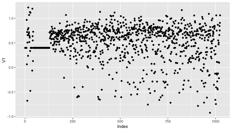
qplot(as.numeric(row.names(hop)),V1,data=hop,xlab = "Index")
qplot(as.numeric(row.names(hop)),V2,data=hop,xlab = "Index")
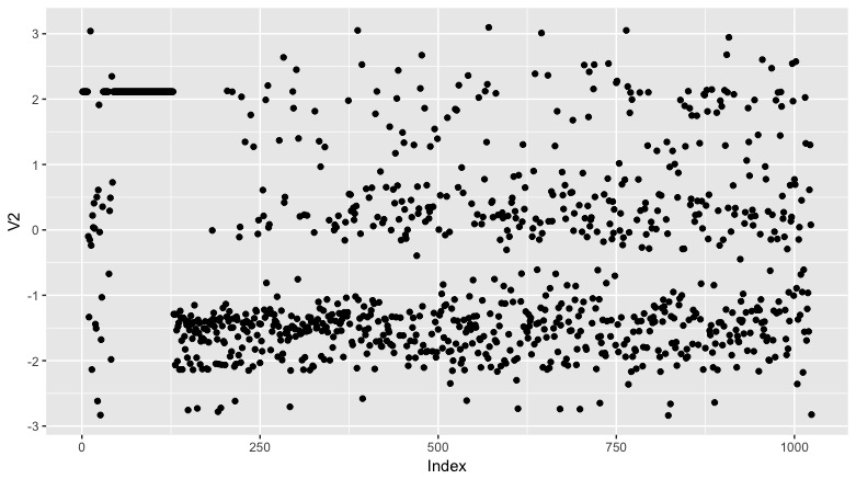
Patterns here. And weird groups of duplicates in both vars between index 0 and 125.
gpairs(hop)
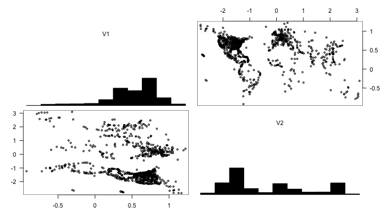
Looks like a world map!
with(hop,qplot(V2,V1))
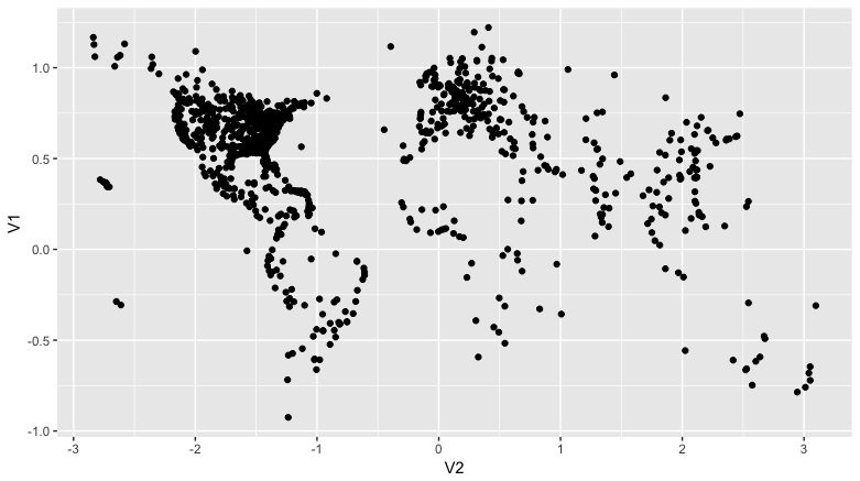
Clearly. Values of 1 on the Y axis appear to correspond to 60 degrees N/S latitude. Maybe all values have been divided by 60?
hop$lon <- hop$V2 * 60
hop$lat <- hop$V1 * 60
lapply(c("ggmap","maps","maptools","mapproj"),require,character.only=T,quietly=T)
basemap <- borders("world")
m <- ggplot() + basemap
m + geom_point(aes(x=hop$lon,y=hop$lat))
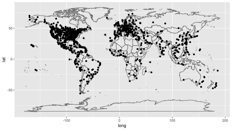
Not quite right. Easting goes beyond 180. Another projection? Looking at different options in Snyder’s manual I don’t think so. But I am reminded that formulas for working with projections are typically done in radians…
names(hop) <- c("v1","v2","lon60","lat60")

180/pi
[1] 57.29578

hop$lonrad2deg <- hop$v2 * 57.29578
hop$latrad2deg <- hop$v1 * 57.29578
m + geom_point(aes(x=hop$lonrad2deg,y=hop$latrad2deg))
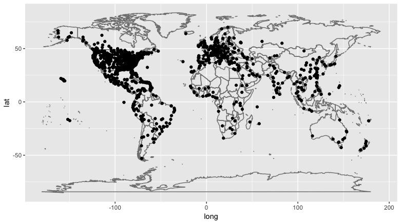
Nice! What about the duplicates?
coordsn <- count(hop,lon = lonrad2deg, lat = latrad2deg)

summary(coordsn)
      lon               lat               n
 Min.   :-162.60   Min.   :-53.00   Min.   :  1.000
 1st Qu.: -92.83   1st Qu.: 19.75   1st Qu.:  1.000
 Median : -73.10   Median : 36.08   Median :  1.000
 Mean   : -37.97   Mean   : 29.63   Mean   :  1.119
 3rd Qu.:  13.26   3rd Qu.: 43.46   3rd Qu.:  1.000
 Max.   : 177.44   Max.   : 69.98   Max.   :101.000

unique(coordsn$n)
[1]   1   2 101

dupset <- data.frame(subset(coordsn,n>1))

str(dupset)
'data.frame':   10 obs. of  3 variables:
 $ lon: num  -150 -122.4 -96.2 -86.3 -82.6 ...
 $ lat: num  61.2 37.6 19.1 39.7 38.4 ...
 $ n  : int  2 2 2 2 2 2 2 2 2 101

dupset[dupset$n > 2,]
       lon    lat   n
10 121.102 22.755 101

m + geom_point(aes(x=dupset$lon,y=dupset$lat))
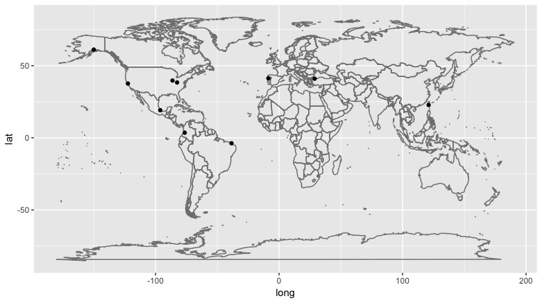
Weird. Seemingly no connection between locations with duplicates. Coming from hopper, I assume these are airports. I can plot points against OSM or similar basemap to confirm. But what is going on with the one in what looks like Taiwan with 101 of them? Maybe something like search traffic on hopper’s servers at a given moment. China’s population is so large that it’s possible.
Unfortunately, no more time for this right now. A future post…